Excel Formatting
Formatting cells
Formatting means changing the appearance of cells, for example you could:
- Change to a larger font size
- Make text and numbers bold, italics or underlined
- Add a currency symbol to numbers - £5.00 instead of 5
- Add borders and shading
Formatting does not affect the actual data in the cell. You can change the formatting of one cell or multiple cells at the same time, but first you would need to select the range of cells that you want to adjust (see above for how to select cell ranges).
Formatting using the Home ribbon
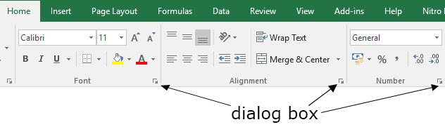
The Font, Alignment and Number sections on the Home ribbon are used to change the format of cells. Each of these sections has a dialog box button at the bottom right which gives you access to more controls.
top of page
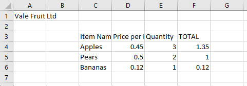
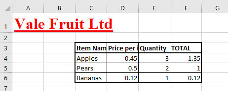
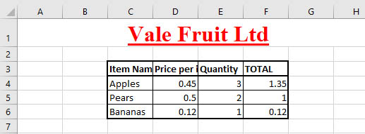
Example: Vale Fruit Ltd
This is a simple spreadsheet that we can improve using formatting changes. Remember that we want to make the sheet easy to understand for anyone using it.
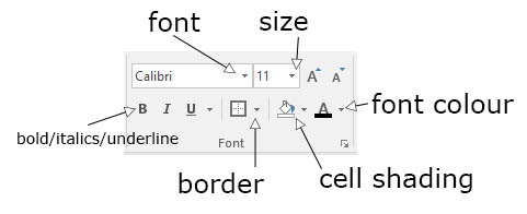
Font
The first thing we'll do is to use the Font section of the ribbon to make the title and headings stand out.
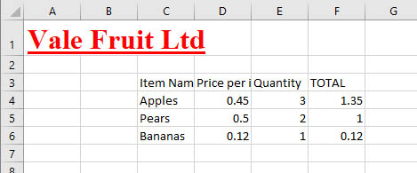
Title
- Click on cell A1
- Change the font to Times New Roman and the size to 24
- Click the B and U buttons to make the title bold and underlined
- Change the font colour to Red
The spreadsheet should now look as below:
Next, we'll make the headings bold and apply a border:
Headings
- Click and drag from C3 to F3
- Click the B button to make all headings bold
Border
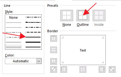
- Click and drag from C3 to F6
- Click the drop-down arrow next to the border button and choose More borders at the bottom of the list
- Click a thick line style then click the Outline preset
- Click a thin line style then click the Inside preset
- Click the OK button at the bottom of the dialog box
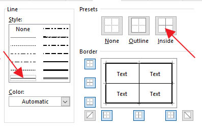
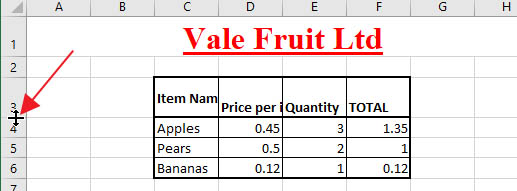
Next we'll give the top row a thick border
- Click and drag from C3 to F3
- Click the Borders button and select More borders
- Click a thick line style then click the Outline preset
- Click the OK button at the bottom of the dialog box
The spreadsheet should now look as below:
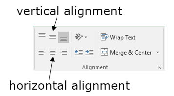
Alignment
Next, we'll have a look at the Alignment section of the Ribbon.
Merge and Centre
- Click and drag from A1 to H1
- Click the Merge and Center button on the toolbar
The cells from A1 to H1 have now been merged into one large cell and the title has been centred across this cell.
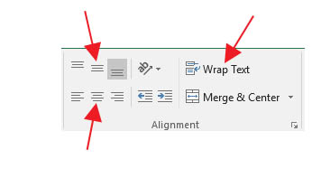
Wrap Text
Some of the headers aren't wide enough to display the text they contain, but instead of making the columns wider we'll allow text to run on to the next line - text wrapping. First we need to make the row taller so that two lines of text can be seen
- Click and drag to make row 3 double the height
- Click and drag from C3 to F3 to highlight the header row
- Click the Wrap text button on the ribbon
- Click the Centre vertical alignment button
- Click the Centre horizontal alignment button
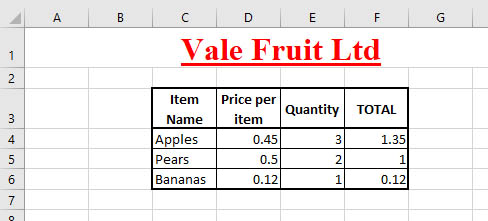
The spreadsheet should now look like this, with the header row showing 2 lines centred horizontally and vertically:
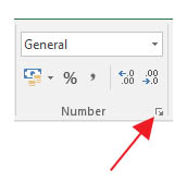
Format numbers
Next, we'll format the price and total cells as currency.
- Click and drag from D4 to D6
- Click the Dialog box button on the Number section of the ribbon
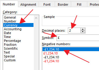
- Click the Currency category on the list. There are options for the number of decimal places, symbol and how negative numbers appear but you can leave these at the default values.
- Click and drag from F4 to F6 and format these values as currency as above
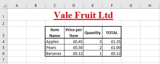
The Spreadsheet should now look as below:
top of page