Excel
Introduction
The term spreadsheet comes from record keeping, where columns of figures would spread across 2 sheets (or pages) of the ledger book.
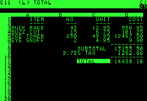
Computer spreadsheets have been around in various forms since the 1960s, but the first modern spreadsheet would probably be VisiCalc which was introduced in 1979. As you can see, the spreadsheet is a grid of columns and rows. Each column has a letter at the top and each row has a number at the left hand side. so each box (or cell) in the spreadsheet has its own unique address given by the column letter and row number.
For example:
- Cell A1 contains the word ITEM
- Cell B5 contains the number 250
There are similarities between ledger books and computer spreadsheets:
- columns of figures
- labels that hopefully tell you what each of these figures mean
- calculations working out sub-totals, totals etc
An advantage of the computer spreadsheet is that it can do all the calculations for you, so you don't have to do any arithmetic! Spreadsheets have found their way into most businesses and organisations so being able to use them competently is becoming essential in the modern workplace.
Microsoft Excel
Excel is part of Microsoft Office (along with Word, PowerPoint, Access and others) and is probably the industry standard spreadsheet at the moment. If you've used another Office program before, you'll find the layout and some features are familiar - saving, printing, formatting etc.
To start Microsoft Excel
This should work if you have Windows 7 or later.
- Click the Start button (or press the Windows key on your keyboard)
- Type in Excel to search for it
- Click on Microsoft Excel from the search results
Excel should now start up.
top of page
The Excel window
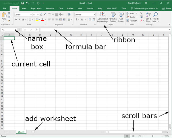
When you open Excel, you'll see a window like the one above (this is the Office 365 version, yours might look slightly different but they all do the same basic tasks).
- The Ribbon is at the top of the window. This will be familiar if you've used another Office program like MS Word, and some of the same formatting controls are there. As you can see, there ribbons for File, Home, Insert, Formulas, Data and so on.
- Below this, you'll see a grid with a letter at the top of each column and a number at the left of each row. Each cell in the grid has its own unique address such as D12, F8, M120 etc.
- The current cell selected will have a border around it (with a square at the bottom right corner). In this case, it's A1
- The name box shows which cell is currently selected (A1 in this example). The current column letter (A) and row number (1) will also be highlighted.
- The formula bar shows the contents of the currently selected cell. If the cell contains a formula, the formula itself will appear in the formula bar and the result of that formula will appear in the cell.
- There are 2 scroll bars in Excel. In the example above you can see columns A-P and rows 1-29, use the scroll bars to see more columns and rows - there are over 16,000 columns and 1,000,000 rows (this means there are more than 16 billion cells in the spreadsheet).
- An Excel file is a workbook which can contain one or more worksheets (spreadsheets). Currently this workbook only has one worksheet (Sheet 1) but you can add more using the button at the bottom left.
top of page
Excel Basics
Select a cell
There are a few ways to move from one cell to another:
- Click with the mouse on the the cell you want to select
- Use the arrow keys on your keyboard to move up, down, left or right
- Press the Enter key to move down one cell - handy if you're entering a column of figures.
Remember that you can check which cell is currently selected by looking at the name box or at the highlighted column letter and row number.
Enter data in a cell
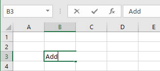
Once you have clicked on a cell, you can start typing to enter some contents to that cell. When you start typing, Excel goes into edit mode so be aware that some features might not be available or might not behave the way you would normally expect. You should see a cursor in the cell as you type, just as you would with Microsoft Word.
When you have finished typing, you can come out of edit mode by:
- Clicking the tick at the left of the formula bar if you want to keep the cell contents that you just typed (the tick and cross only appear in edit mode)
- Clicking the formula bar cross if you want to delete what you just typed
- Pressing the Enter key (this will also move to the cell below)
Change the contents of a cell
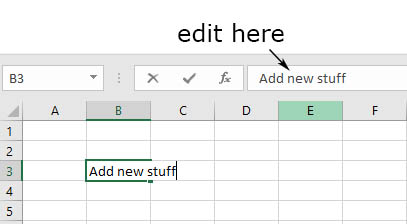
Cell contents will be displayed in the cell itself and also in the formula bar. An easy way to change a cell is to use the formula bar.
- Click on the cell whose contents you want to change
- If you want to replace the entire contents, just start typing and the existing text will be deleted
- If you just want to change part of the contents, click inside the formula bar and make the required changes
- When you're finished, press Enter or use the tick/cross buttons to come out of edit mode.
Adjust column width and row height
You can make columns wider and rows taller if required. Sometimes this is not necessary - if the contents of cell A1 overlap into B1 they will still be visible provided there is no data in B1. And the spreadsheet contains billions of cells so you could easily leave B1 blank, whereas widening column A would make every cell in that column wider so would hide part of the column on the far right.
If you do need to adjust column and rows
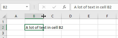
In this example, there's a lot of text in cell B2 which overlaps into C2. To make B2 wider:
- Move the mouse pointer between the column B and C header buttons till the cursor changes to a black double-headed arrow (as shown below)
- Click and drag the mouse to the right till the column is wide enough
- You could also double-click instead of click and drag - the column width will automatically fit the widest cell contents
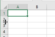
Row height can be adjusted the same way - move the mouse pointer between the row numbers at the left hand side till you get a double-headed arrow.
Data Types
There are 3 types of data that you can put into an Excel cell: text, numbers or formulas.
Text
Text can be used to show what the numbers mean, like putting 'Sales' at the top of a column so that anyone who sees the spreadsheet will know what that column of numbers means. Spreadsheets can also be used to store records - names, addresses, product details and so on - and these will be stored as text.
Numbers
Numbers could be prices, quantities, ages, years etc. Cells with numbers in them can have calculations performed on them by the spreadsheet so make sure you don't include any text along with the numbers - don't put '56 pence' in a cell.
Formulas
Cells with formulas are a bit different because the formula itself won't be shown in the cell, instead you'll see the result of that formula. For example, you could enter a formula that adds the numbers in 2 other cells and shows the total.
top of page
Excel formulas
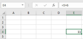
Excel formulas always start with the equals symbol =. If the first thing you type into a cell is the equals symbol, excel knows this is going to be a formula and treats the cell differently to text and number cells.
This may seem a bit backwards at first, because we're used to seeing the equals symbol before the result: 1+1=2
In this example, I clicked in cell E4 then typed the formula =5+6 and clicked the tick at the left of the formula bar (so I came out of edit mode and stayed on cell E4). Cell E4 shows the result of the formula (11) but if you look at the formula bar you can see the formula I typed in =5+6.
Cell references
Another way to do this would be to put the numbers 5 and 6 in separate cells then use the addresses of those cells in the formula. This can be very useful!
This time, the formula in E4 is =C4+D4
Excel looks at the contents of C4 and D4, adds them together and shows the result in E4.
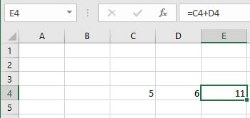
This means whenever I change the numbers in C4 and D4 (and come out of edit mode), Excel will automatically add the new numbers and show the result in E4.
Arithmetic operators
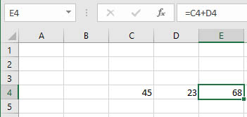
As shown above, Spreadsheets use the plus symbol for addition. Of course, we can also subtract, multiply and divide:
- The plus is used for addition =C4+D4
- The hyphen is used for subtraction =C4-D4
- The asterisk (star) is used for multiplication =C4*D4
- The forward slash is used for division =C4/D4 would be C4 divided by D4
- The caret symbol ^ is used for exponents =3^2 would be 3 squared
Order of precedence
You might see a formula with more than one operator like =3+2*5. What's the answer?
You might look at the operators in order from left to right so:
- 3 + 2 is 5
- 5 times 5 is 25
- so the answer is 25
But Excel gives the answer as 13!
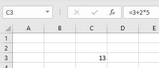
This is because Excel follows the mathematical order of operations - sometimes this is called BODMAS. In order this would be:
- Brackets - anything in ()
- Orders like squares or square roots
- Division
- Multiplication
- Addition
- Subtraction
Looking back at the formula =3+2*5 this means multiplication is carried out before addition, so:
- 2 times 5 is 10
- 3 plus 10 is 13
- So the answer is 13
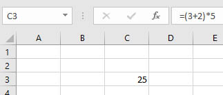
Remember that anything in brackets would be calculated first, so if you wanted to add 3+2 first then multiply the answer by 5 you would write =(3+2)*5
Showing Formulas
Formulas are hidden in Excel - the cell shows the result of the calculation. You could click on the cell containing the formula and view it in the formula bar but this would only show one formula at a time.
You might want to see all the formulas in a sheet, or print the sheet showing formulas. To do this:
- Click on the Formulas tab on the Ribbon
- Click Show Formulas in the Formula Auditing section
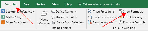
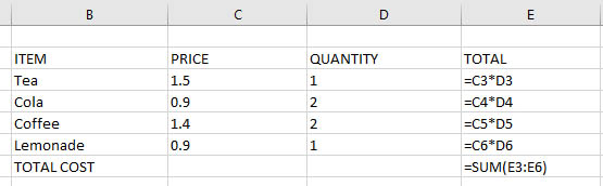
The formulas in the worksheet will now be visible (click the Show Formulas button again to hide them).
top of page
Functions
Formulas look very useful, but what if you wanted to add a column of numbers...and there were a lot of numbers in the column? You would have to have a formula like
=E4+E5+E6+E7
and so on. This might take a while to write and it would be easy to make a mistake. Fortunately, there's an easier way - using functions.
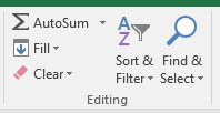
Autosum
In this example, we'll add a column of numbers using the Autosum function which has a button at the right of the Home ribbon
First, type a list of numbers in the spreadsheet then click in the empty cell below the list:
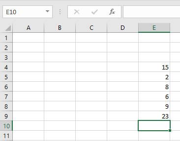
Then click the Autosum button, you should see the SUM function as below:
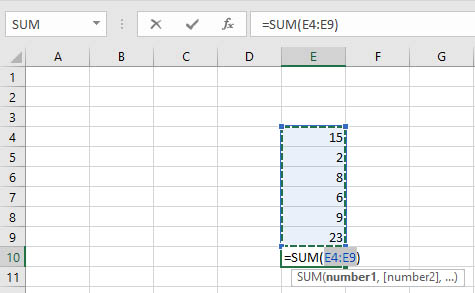
The function that was automatically put in the cell is =SUM(E4:E9)
E4:E9 is a cell range, this makes it easier to refer to a large column or row of cells.
If the function looks OK, click the tick or press Enter to come out of edit mode and see the result.
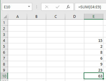
So, the total of this column is 63
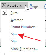
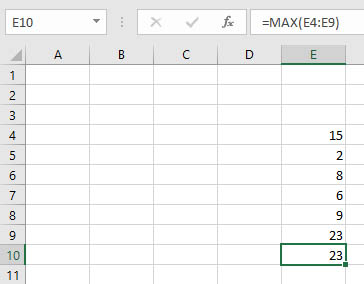
Max
The Max function is used to find the maximum (or highest) value in a cell range.
Example
- Click the cell below a column of numbers (or next to a row)
- Click the drop down arrow at the right of the Autosum button and click Max
- Click the tick or press Enter to come out of edit mode
- The function is =MAX(E4:E9) and it has found the highest number, 23
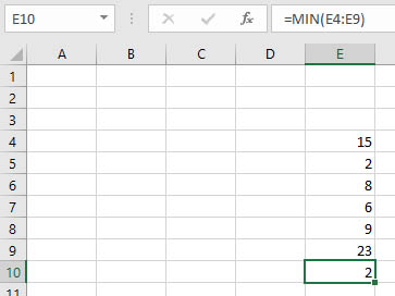
Min
The Min function finds the minimum (lowest) value in a cell range. It is also on the Autosum drop-down list, or you could write it yourself: =MIN(E4:E9)
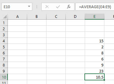
Average
This function works out the average of a cell range, =AVERAGE(E4:E9) in this case. It's also on the Autosum button list.
top of page
Selecting cells
So far, we've looked at selecting one cell at a time which you can do by clicking on the cell, using the arrow keys etc. Sometimes you will want to select a range of cells though, and there are a few different ways to do it.
Click and Drag
Click on the first cell you want to select and drag to the last cell. In the example below, I clicked on cell B2 then dragged down and right to D6.
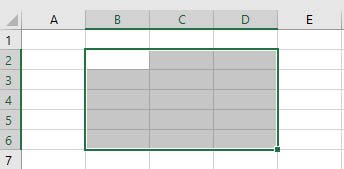
As you can see, there's a border round the cell range B2:D6 and all of these cells are now selected (the first cell has a white background but ignore this - they're all selected.
Click and Shift-Click
Another way to do the same thing without dragging:
- Click on cell B2
- Hold down the Shift key
- Click on cell D6
- Release the Shift key
The same cell range will be selected.
Alter a selection
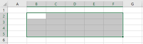
You can extend or reduce a selection by holding the the Shift key and using the arrow keys on your keyboard. As an example, we'll extend the selection by 2 columns and reduce it by one row:
- Hold down the Shift key
- Press the right arrow twice
- Press the up arrow once
- Release the Shift key
The new selection will be from B2:F5.
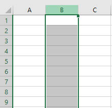
Select an entire column or row
If you want to select every cell in a column or row, click on the column letter at the top of the column or on the row number at the far left.
Example
Click on the B button at the top of row B. All the cells in this row are now selected (over a million cells!)
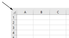
Select every cell in the spreadsheet
Keyboard shortcut
- Hold down theCtrl key
- Tap the letter A
- Release the Ctrl key
Button
- Click the button at the left of Column A and above Row 1
Non-adjacent selections
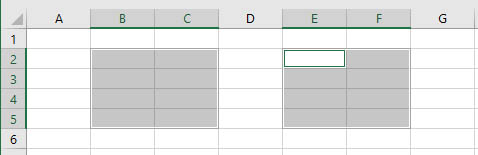
Sometimes you might want to select ranges of cells that aren't next to each other - for example B2:C5 and E2:F5
You can do this with the Ctrl key:
- Click on cell B2 and drag to C5
- Press and hold the Ctrl key
- Click on cell E2 and drag to F5
- Release the Ctrl key
You now have 2 cell ranges selected at the same time.
top of page
Inserting Rows and Columns
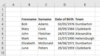
You can insert extra cells, rows and columns into your spreadsheet if necessary. For example, have a look at the spreadsheet below:
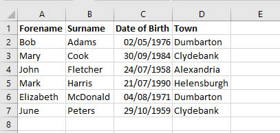
There isn't room for a title in cell A1 and we want to add a column for middle name. Also, the records are alphabetical by surname but suppose we have to add someone between Mary Cook and John Fletcher?
Example - insert rows and columns
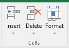
First, we'll move the data 2 rows down and one column to the right to give room for a title. We'll use the Cells section of the home ribbon for this.
- Click on cell A1
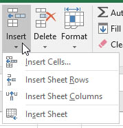
- Go to the Cells section of the ribbon and click the drop-down arrow below Insert
- Click Insert Sheet Rows
- You should see that a blank row has been inserted in Row 1 and all the data in Row 1 and below has been moved down
- Click the drop-down arrow then Insert Sheet Rows again to move the data down another row
- Click the drop-down arrow then Insert Sheet Columns again to move the data right one column
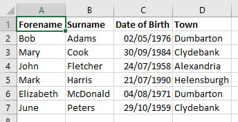
The spreadsheet should now look as below:
Click on cell A1 and add the title Customers
Next, we'll add another person between Cook and Fletcher
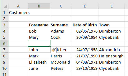
- Click on cell B6 (We could click on any cell in row 6)
- Click the Insert drop-down arrow then Insert Sheet Rows. There should now be a blank row between Cook and Fletcher
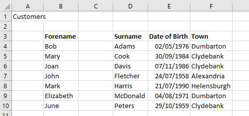
- Put Joan Davis born 7/11/86 from Clydebank in this row
Next, add a column for Middle Name
- Click on cell C6 (or any cell in column C)
- Click the Insert drop-down arrow then Insert Sheet Columns. There should now be a blank column between Forename and Surname
- Type Middle name in cell C3
- Add middle names for some customers
Deleting Rows and Columns
This is similar to inserting
- Click a cell in the row or column that you want to delete
- Click the drop-down arrow below Delete
- Click on Delete sheet rows or Delete sheet columns as required
top of page
Auto Fill
Auto fill is a time saving feature built into Excel, for example you could type in 'Monday' and it will fill in the rest of the weekdays for you
Example
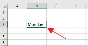
- Type Monday in cell B3 and click the tick to come out of edit mode
- Make sure you're still on cell B3 and notice the fill handle at the bottom right of the cell
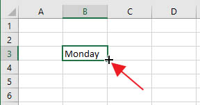
- Move the mouse pointer over the fill handle till the cursor changes to a black plus sign
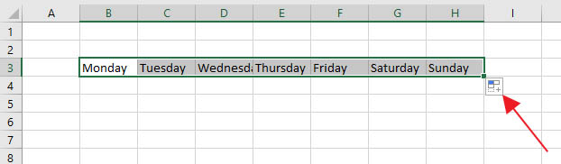
- Click and drag to cell H3 and the rest of the days of the week will be filled in. You should see an Auto Fill Options button when the cells have been filled in.
- If you drag further than H3 the pattern of weekdays would continue repeating Monday-Sunday
Auto Fill Options
The options vary depending on the type of data being filled (numbers, days, dates etc). There are 6 options for weekdays, the first 4 will be available for all auto fill data.
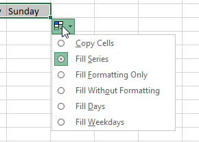
- Copy Cells would copy the value in the first cell, so all 7 cells in this example would show 'Monday'
- Fill Series fills the series of weekdays (or months etc depending on what you typed in the first cell)
- Fill Formatting Only just copies the format (font, bold, alignment etc) of the first cell and leaves the values in the rest of the cells unchanged
- Fill Without Formatting fills the series but doesn't copy the format of the first cell
- Fill Days fills the days Monday-Sunday (including weekends)
- Fill Weekdays only fills Monday-Friday
Filling a series of numbers
You may want to fill a series where the difference is more than 1, for example the 7 times table or the dates of all Fridays in February. To do this, enter the first 2 values in cells then click and drag to highlight both cells before using the auto fill handle.
Example
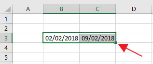
- Type 2/2/2018 in cell B3
- Type 9/2/2018 in cell C3
- Click and drag to highlight cells B3 and C3
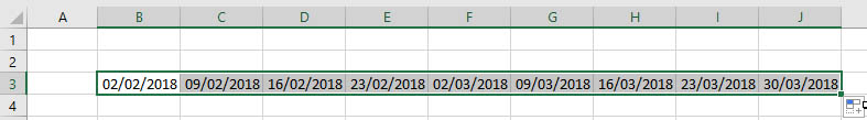
- Click on the auto fill handle (get the black plus cursor first) and drag to cell J3
- The dates of all Fridays from February-March will be filled in
Auto Fill Formulas
A useful way to use auto fill is when you're completing a lot of similar formulas.
Example
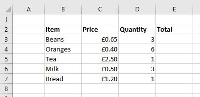
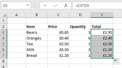
We need to put in 5 formulas here to calculate totals for each item. The normal way to do this would be:
- Enter the formula =C3*D3 in cell E3
- Enter the formula =C4*D4 in cell E4
- ...and so on
To save time we'll use auto fill:
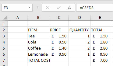
- Click on cell E3 and enter the formula =C3*D3
- Click the tick to come out of edit mode
- Move the mouse pointer to the auto fill handle at the bottom right of the cell
- Click and drag down to cell E7 then release the mouse button
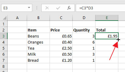
Excel has filled in the formulas for us. It's important to check the formulas to make sure Excel has filled them in correctly.
Absolute and relative cell references
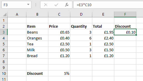
Here's a problem you could run into when using auto fill on formulas. I'm going to apply a 5% discount to each total, and the cell with 5% is C10 so the formula will be =E3*C10.
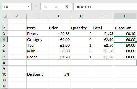
Then I use auto fill to copy the formula down, but it doesn't work - the discounts are zero. I've clicked on F4 to check the formula =E4*C11 and I can see the problem - there's nothing in C11 so E4 x 0 is zero!
What I need to do is make C10 an absolute cell reference in the formula. This means the formula will always use cell C10 even when you use auto fill. I want E3 to change to E4, E5, E6 and E7 so that will remain a relative cell reference.
To make a cell an absolute reference you put a dollar symbol before the column letter and row number - my formula should be =E3*$C$10.
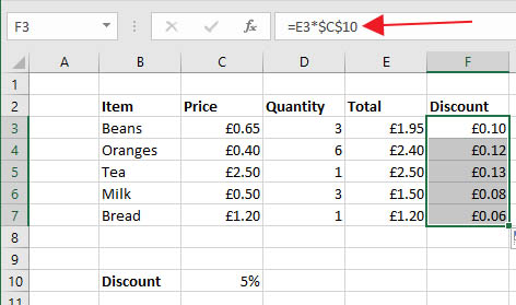
As you can see, this works when I copy it down with auto fill.
Absolute references
- Absolute references don't change when the formula is auto filled
- Put a dollar symbol before the column letter and/or the row number to make a reference absolute
- This means the column and/or the row won't be changed when the formula is auto filled
- You can press the function key F4 when you are typing the cell address to automatically add dollar signs
top of page
Headers & Footers
Headers and footers are useful when you're printing your spreadsheet. Anything put in the header will appear at the top of each page that's printed and anything you put in the footer will appear at the bottom. You can type in text, such as your name, or use buttons to automatically add text like the file name, date, page numbers and so on.
Adding a header or Footer
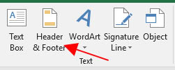
- Click on the Insert ribbon and select Header & Footer in the Text section
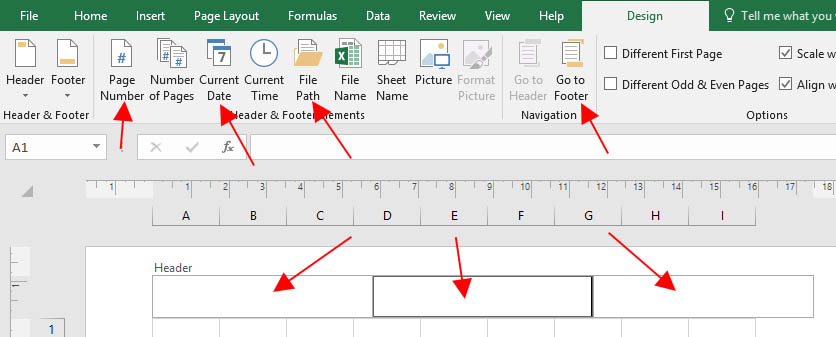
- You will now be able to edit the Header. A New Design tab appears on the ribbon which has buttons that help you make changes.
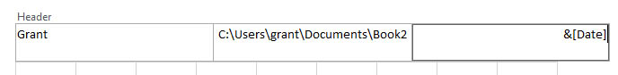
- The header is split into 3 sections - the left, centre and right - and you can add data to each. Click on the left section and type your name.
- Click in the centre section then click the File Path button
- Click in the right section and click the Date button. The header should look as below:
- Click the Go to Footer button on the ribbon
- Click in the right section of the footer then click the Page Number button on the ribbon.
- To close headers or footers, click any cell in the worksheet
- You will be viewing the spreadsheet in Page layout view, to return to normal view click the View tab on the ribbon then click Normal

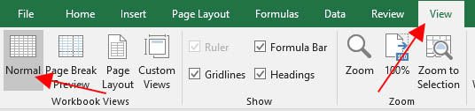
You can check how the header and footer will appear on the printed page by switching to Page Layout view (View tab on the ribbon).
top of page