More Excel
Naming cells and ranges
So far, we've referred to cells by their column and row - for example A1, F58 and so on. Excel also lets you give cells names of your own. This can be useful when writing formulas, instead of typing the cell reference you give the cell a meaningful name and then use that name in the formula. So, instead of:
=C3*B2
You could give cell B2 the name VAT and have a formula like
=C3*VAT
Names can also be applied to cell ranges.
We've already had a look at absolute and relative cell references in the autofill section, note that cell names will be absolute references. This can be handy when you're autofilling formulas.
Rules for creating names:
- The first character of a name must be a letter, an underscore character, or a backslash. Remaining characters in the name can be letters, numbers, periods, and underscore characters.
- Names cannot be the same as cell references (A1, B7 etc)
- Spaces are not allowed as part of a name
- Names are not case sensitive - vat is the same as VAT
Example
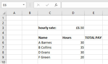
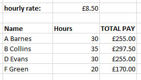
Have a look at the spreadsheet below, we're going to put a formula in cell E6 that will calculate the total pay for each employee. Since we'll use autofill to copy the formula down, we need to make the cells containing pay rates absolute references, so the formula would be:
=D6*$D$3
if we weren't using names.
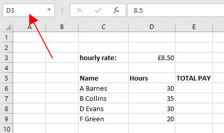
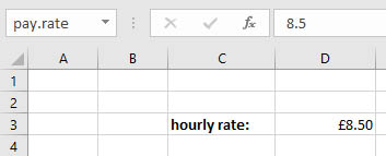
Instead, we'll give cell D3 the name pay.rate and use this in the formula.
- Click on cell D3 to select it
- Click the name box at the top left
- Type pay.rate in the name box
- Press Enter
- Click in cell E6
- Enter the formula =D6*pay.rate
- Press Enter
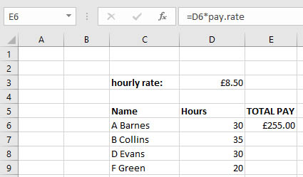
You can use autofill to copy this formula down to calculate total pay for the other employees.
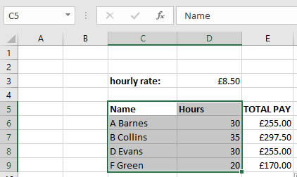
Named ranges
You can give names to cell ranges in the same way - this could be useful for selecting data for charts or for lookup functions.
- Click and drag fron C5 to D9
- Click in the name box
- Type hours.worked
- Press Enter
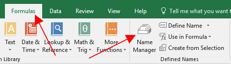
Editing names
If you want to change or delete a name:
- Click the Formulas ribbon
- Click the Names manager
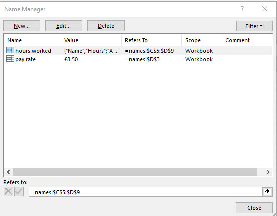
- This will give you a dialog box that lets you select the current names and delete them or make changes.
- For example you could click on hours.worked then Click the Edit button to change the name or cell range
Scope
By default, the scope of these names is workbook. This means you can use the names to refer to these cells/ranges from any sheet in the workbook. You can change the scope to worksheet, in which case you wouldn't be able to use it in other sheets since its use is restricted to the current sheet. Names have to be unique in their scope, so you can't have another sheet in the workbook with a cell called pay.rate.
top of page
More functions
If
The If function lets you choose what action to take depending on whether a condition is met. The basic format is:
IF (Something is True, then do something, otherwise do something else)
For example, we could check whether a score is greater than or equal to 50 (our condition) then assign a pass or fail grade
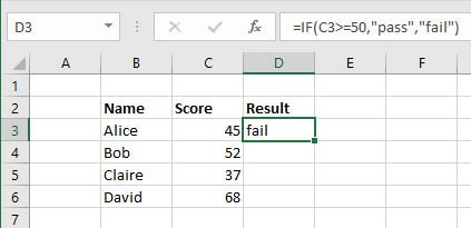
- The function starts with =IF(
- The score for Alice is in C3 so our condition will be C3>=50
- Next, a comma
- If this is true we want to show a pass so put this in quotation marks"pass"
- Another comma
- If the score is below 50 we'll show the word "fail"
- Finally a closing bracket )
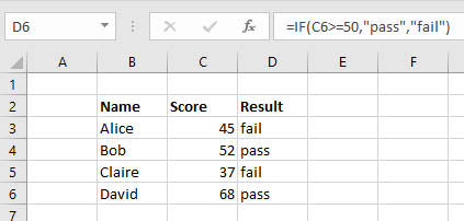
Copying the formula down, we would get results for everyone:
Comparison operators
| Comparison | Operator | Example | Meaning |
|---|---|---|---|
| Equal to | = | A1=B1 | A1 equals B1 |
| Less than | < | A1<B1 | A1 is less than B1 |
| Greater than | > | A1>B1 | A1 is greater than B1 |
| Greater than or equal to | >= | A1>=B1 | A1 is greater than or equal to B1 |
| Less than or equal to | <= | A1<=B1 | A1 is less than or equal to B1 |
| Not equal to | <> | A1<>B1 | A1 is not equal to B1 |
VLOOKUP
The VLOOKUP function can be used to find information in a specified row in a table. For example you might look up someone's name in a telephone directory to find their phone number. This function looks quite complicated but it can be very useful once you get the hang of it. The basic format is:
=VLOOKUP (value you want to look up, cell range, column where you want the value returned, FALSE for exact match or TRUE for approximate match)
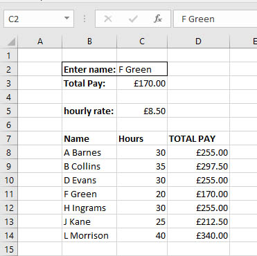
Example
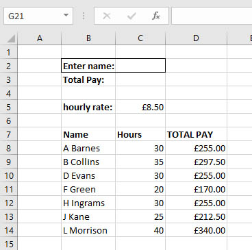
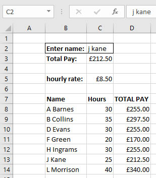
Here we have a table B8:D14 showing name, hours and total pay. I want to be able to type a name into cell C2 and have the total pay for that person shown in cell C3. The VLOOKUP function can do this, but it needs 4 pieces of information for it to work:
- The value I want to look up will be typed into cell C2
- The cell range is B8:D14
- There are three columns in this range, total pay is in the third column so I need to put 3 in the function
- I want an exact match so FALSE
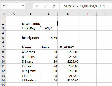
So, to enter the function:
- Click in cell C3
- Type the function =VLOOKUP(C2,B8:D14,3,FALSE)
- Press Enter
- I haven't typed a name in yet so the value in C3 is showing as not available (N/A)
- Type a name from the list and check the correct pay is shown in cell C3
It's possible to use named ranges in the formula - I could have selected B8:D14 and given it the name pay for example. Then the function would be:
=VLOOKUP(C2,pay,3,FALSE)
top of page
Sorting data
Basic sort
When you sort data, you put it into an order that makes it easier to use. For example we could put a list of products in alphabetical order or order a list of prices from lowest to highest.
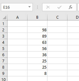
Here's a list of 8 numbers, we'll order them from highest to lowest.
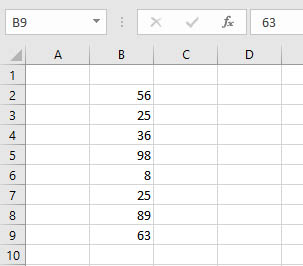
- Click a cell in the column you want to order, for example B2
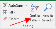
- Click Sort & Filter on the Editing section of the Home ribbon
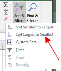
- We'll choose Sort Largest to Smallest because we want them ordered from the highest number to the lowest.
- The list is now ordered from the highest to the lowest number
You can also use this to sort lists of words or dates.
Sorting more than one column
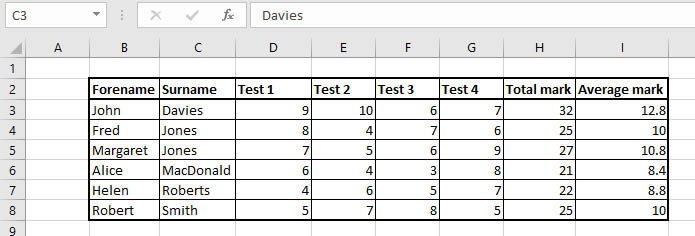
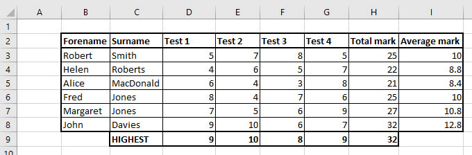
The above method is fine if you've only got one column of data, but we've often got data across multiple columns as below:
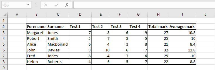
Suppose we want to sort alphabetically by surname, we would use the same method as above but what happens to the data in the other columns - will it also be reordered?
- Click C3
- Click Sort & Filter
- Choose Sort A to Z
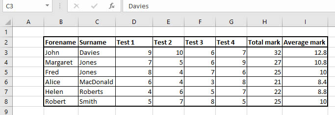
As you can see, the other columns have been sorted along with the surname column. But there are 2 people with the surname Jones and we would prefer them to be sorted alphabetically by forename - Fred should be before Margaret.
Add Sorting Levels
We can do this by adding sorting levels. The first level will be Surname then the next level Forename will be used for records whose surnames match.
- Click C3
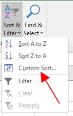
- Click Sort & Filter
- Choose Custom Sort...
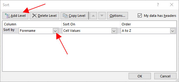
- This gives us a dialog box that lets us add levels. Click the drop-down arrow next to Forename and change this to Surname since that will be our first level. Then click the Add Level button
- Use the drop down arrow to change the sorting on the new level to Forename
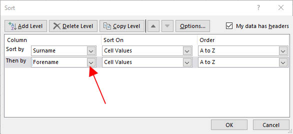
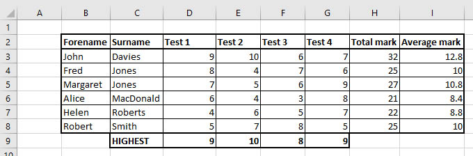
The table is now sorted alphabetically by Surname, then by Forename:
Selecting a range to sort
Sometimes it's necessary to select the range you want sorted, for example if there's a row at the bottom of the table that should always stay at the bottom. You might have noticed on the Custom Sort dialog box that there's an option to include a header row:
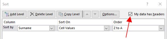
This stops the top row with Forename, Surname, Test 1 and so on being sorted with the rest of the data. But what happens when there's a row at the bottom that shouldn't be sorted?
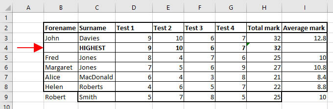
If you click on cell C3 and sort by surname, the bottom row is included with the other rows:
To prevent this, click and drag to select the cell range that you want to be sorted before choosing the sort method. In the above example, this would mean selecting the cells B2:G8 before sorting (this includes a header row).
The data is now sorted correctly.
top of page
Working with multiple worksheets
Excel spreadsheets come in the form of workbooks which can contain several worksheets. You can add additional worksheets and rename them to give you an idea of what's on each sheet. You can also reference cells on other worksheets, although you would obviously have to make it clear which worksheet and cell you were referencing.
Adding worksheets
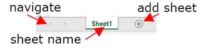
The button to add a worksheet is at the bottom left of the spreadsheet, click this and another sheet will be created. Currently there is one sheet in this workbook, called Sheet1. Click this and there will be another sheet called Sheet2.

Renaming worksheets
We'll rename these sheets, one is for data relating to 2018 and the other is for 2019 so we'll just call them the years.
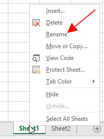
- Right-click on Sheet1
- Select Rename from the context menu
- Type 2018
- Press Enter
- Do the same for Sheet2, except call it 2019

Referencing cells in other worksheets
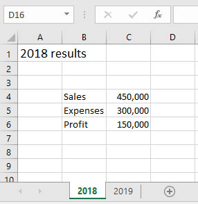
Click on the 2018 worksheet and enter the data as below:
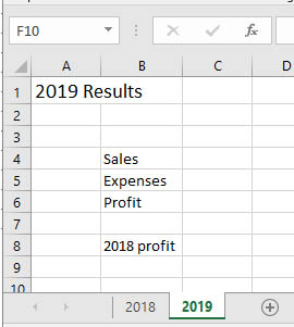
Then click on the 2019 sheet and enter the following:
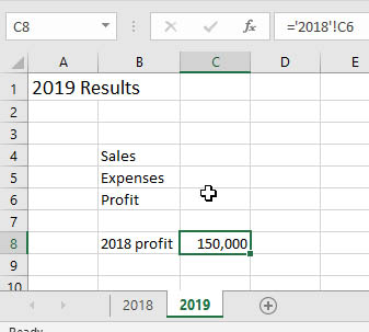
We want to get the profit from cell C6 in the 2018 sheet and put it into cell C8 in the 2019 sheet, but if we type =C6 in C8 it will take the C6 value from the 2019 cell which is blank. So how can we do this?
To reference a cell in another sheet, put the sheet name followed by an exclamation mark before the cell reference.
- Click on cell C8 in sheet 2019
- Type =2018!C6
- Press Enter
- The value from sheet 2018 cell C6 will now be in cell C8
top of page
Protect worksheets
You can prevent other people making changes to your worksheet by protecting it. This can stop others accidentally deleting parts of the sheet, changing formulas etc. You can also choose cells that other people are allowed to edit and protect the rest of the sheet. There are 2 steps to this:
- Select the cells you want to be unlocked (editable)
- Protect the sheet
Using the sheet with a VLOOKUP function as an example, I want to allow people to enter a name to find out the total pay for that employee but I want to protect the rest of the sheet so that nobody can change it.
1 Unlock cells
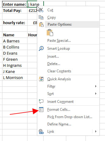
- Click on the cell or cells that you want to unlock - C2 in this case
- Right-click on the cell (or in the cell range) and select Format Cells
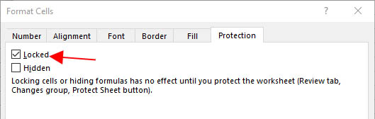
- Click in the Locked checkbox to remove the tick so that this cell (or range) will not be locked
- Click OK at the bottom right of the dialog box
2 Protect the worksheet
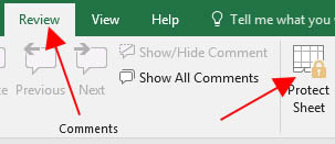
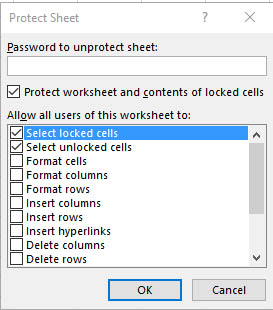
- Click the Review tab on the ribbon then click the Protect Sheet button
- Enter a password if required then choose what actions are allowed - by default users can select locked and unlocked cells (but not enter any data in them)
- Click OK at the bottom of the dialog box
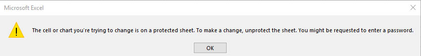
The sheet is now protected, if anyone tries to enter data in a cell other than C2, they will get an error message
top of page